You can format tables and crosstabs based on conditional IF statements. The IF condition is based on the value of the column data.
- Click in a column of a table.
- Click Table
Formatting.

- In the Table
Formatting panel, click IF Conditional.

The Conditional Formatting menu opens. Visualizer lists the columns you can format. You can enable or disable formatting after you define it.
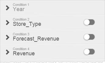
- To define
the formatting, click a condition. Visualizer displays the basic
formatting options for the type of data in the column.Tip: If basic formatting options do not apply to the data, Visualizer displays the advanced formatting options, where you can add an expression.
- In basic formatting,
format the data using one, two, or three intervals. The default
is one interval.

You can add an icon and change the color of the data in the cell.
Example: A quantity over a specified amount can display a green up arrow.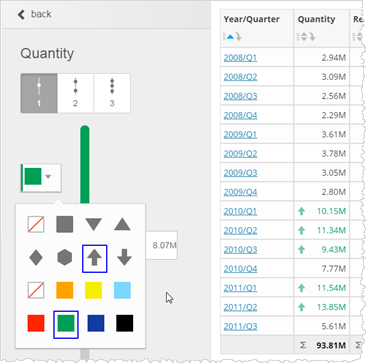
- Use the slider to set the conditional threshold.
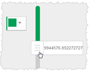
You can also format the values below the threshold.
Example: You can specify a color and icon for low values. This formats every cell.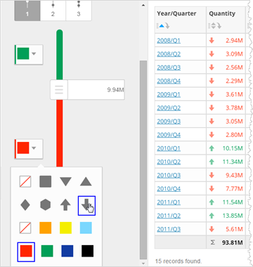
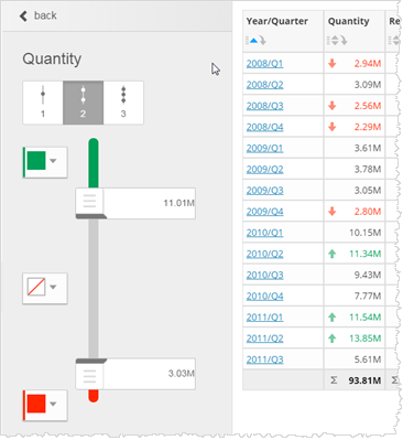
- Click the Interval
icon for two or three intervals to add additional formatting or leave some cells unformatted.Example: To add formatting to only the upper and lower ranges, select two intervals and format them.
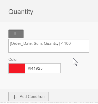
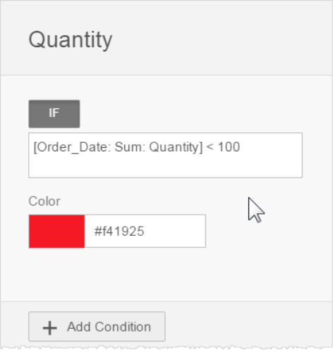
- Use advanced formatting and add an expression or multiple expressions.
Assign each expression a color and/or an indicator icon, and click Apply.
- When you are
finished defining conditional formatting, click Done.